Quick Navigation:
| | | |
Statistics
17.1 Introduction
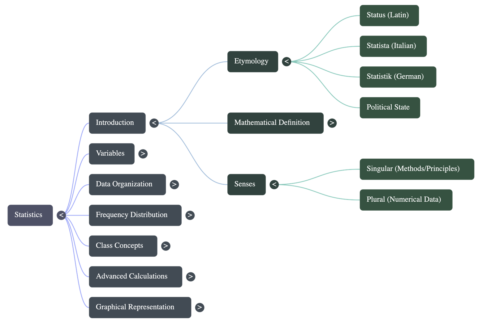
- Origin of the Word: The term "Statistics" originated in the mid-18th century from the Latin word 'Status', Italian word 'Statista', or German word 'Statistik', all meaning a 'Political State'.
- Two Meanings of Statistics:
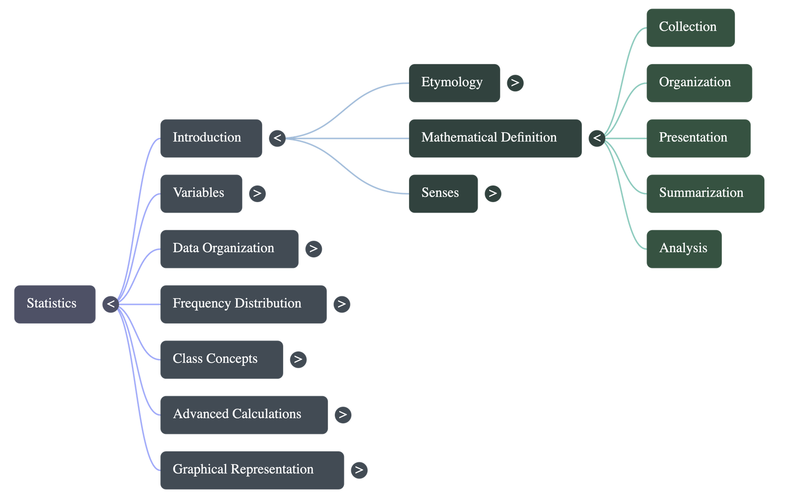
- Singular Sense: It refers to the subject or branch of mathematics dealing with the collection, organisation, presentation, summarisation, and analysis of data to draw conclusions.
- Plural Sense: It refers to the actual numerical data collected systematically for a specific purpose (e.g., marks of students, unemployment numbers).
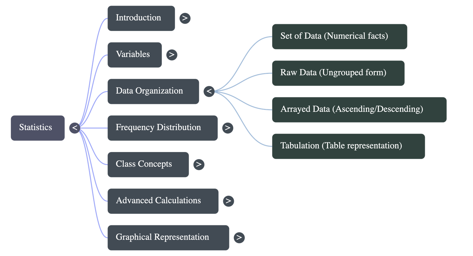
- Data: A collection of numerical facts gathered with a definite object in view is called a set of data.
17.2 Variable
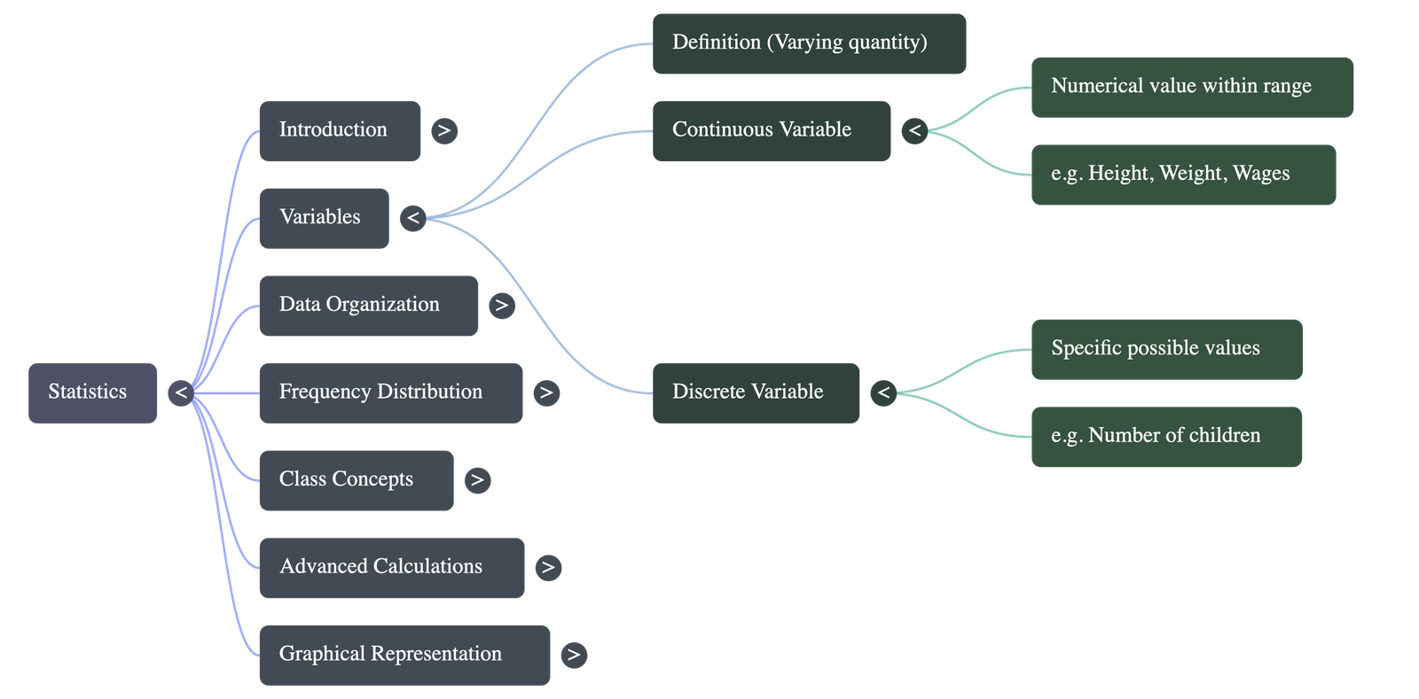
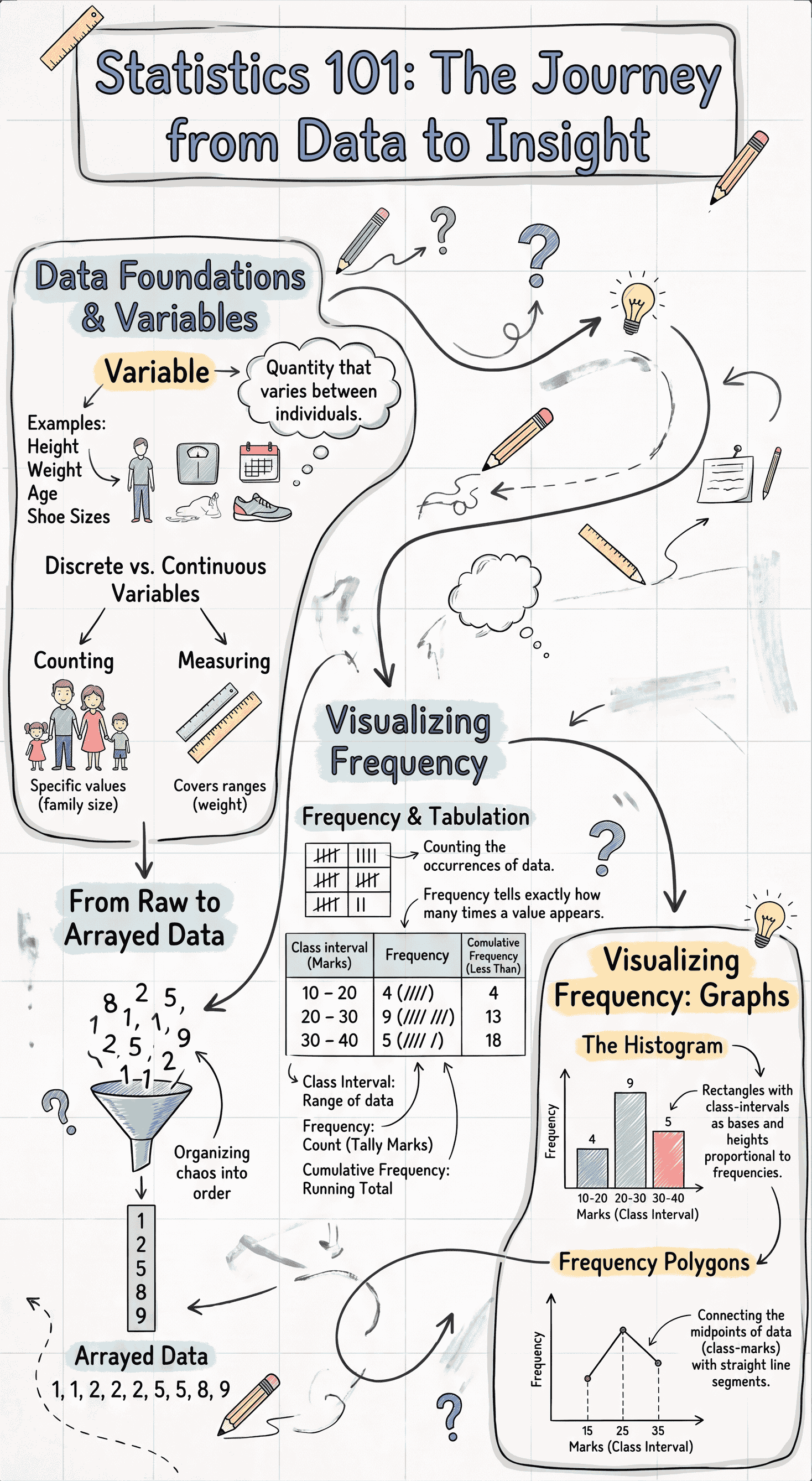
- Definition: A quantity that can change or vary from one individual to another (like height, weight, or age) is called a variable.
- Continuous Variable: A variable that can take any numerical value within a given range, including decimals (e.g., heights of children, rainfall records).
- Discrete Variable: A variable that cannot take all possible values and usually jumps from one whole number to another (e.g., the number of children in a family cannot be 2.5).
- Raw vs. Arrayed Data: Unorganized data is called raw or ungrouped data. When this data is arranged in ascending or descending order, it becomes arrayed data.
17.3 Tabulation of Data
- Definition: The process of representing collected facts and numerical data systematically in the form of a table (with rows and columns) is called tabulation. This makes data easy to read and understand.
17.4 Frequency
- Definition: Frequency is simply the number of times a particular piece of data appears in a given set. For example, if the number '2' appears four times in a test score list, the frequency of '2' is 4.
17.5 Frequency Distribution
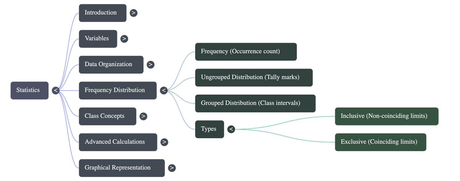
- Definition: A table that pairs data values with their corresponding frequencies is called a frequency distribution table.
- Ungrouped Frequency Distribution: Used for smaller data sets. We list the exact items (like shoe sizes) and use Tally Marks (strokes) to count their frequencies. Every fifth stroke crosses the previous four to make a bundle of five, making counting easier.
- Grouped Frequency Distribution: Used for larger data sets. The data is condensed into groups called class intervals (e.g., 1–10, 11–20) rather than listing every single number.
17.6 Types of Frequency Distributions
- Inclusive Distribution: The upper limit of one class interval does not overlap with the lower limit of the next (e.g., 1–10, 11–20). The number 10 is included in the 1–10 group.
- Exclusive Distribution: The upper limit of one class interval is the exact same as the lower limit of the next (e.g., 10–20, 20–30). Important rule: The upper limit value is excluded from that class. So, a mark of '20' belongs to the 20–30 group, not the 10–20 group.
17.7 Class Intervals and Class Limits
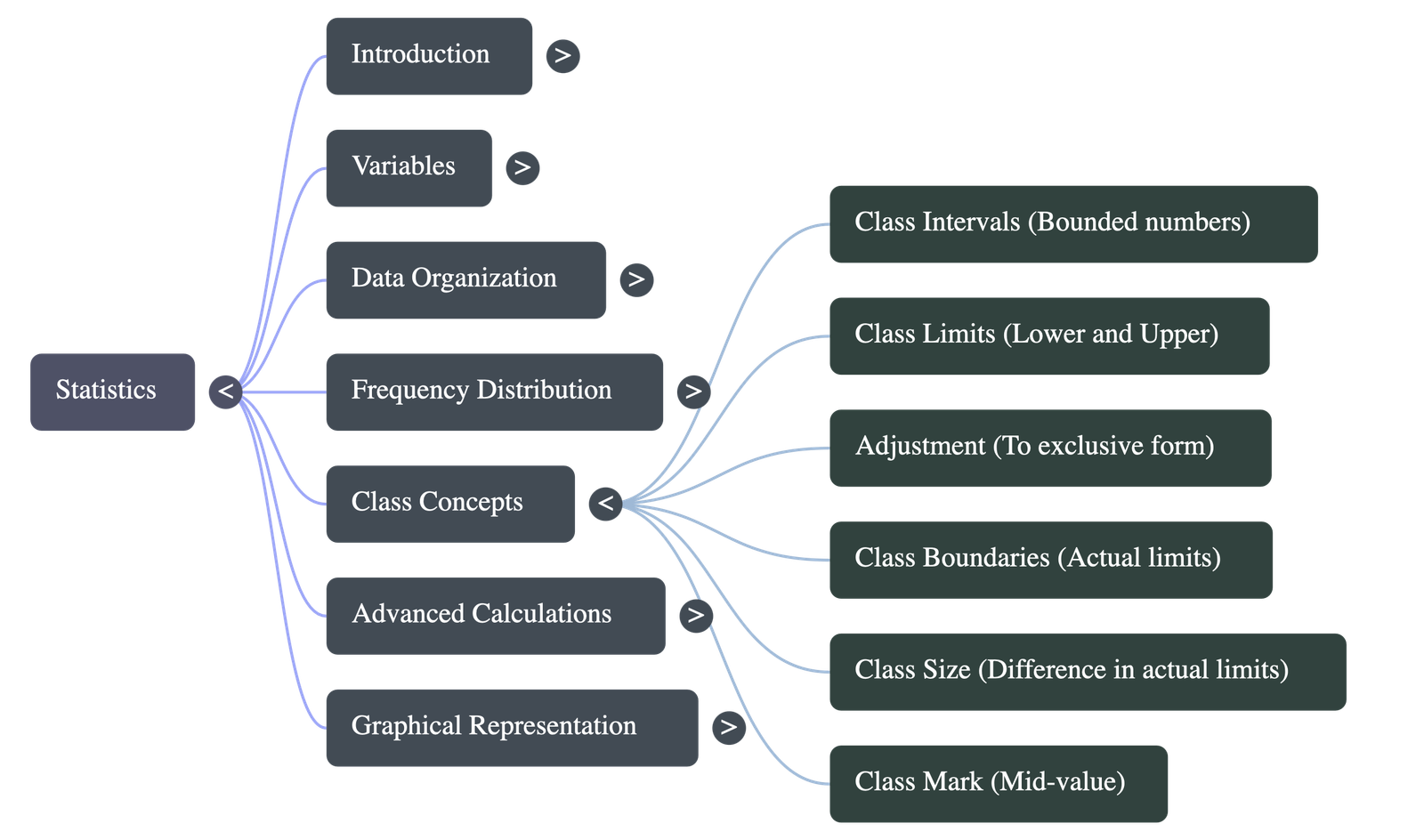
- Class Limits: The two numbers forming the boundaries of a class interval (e.g., in 10–20, 10 is the lower class limit and 20 is the upper class limit).
- Adjustment (Converting Inclusive to Exclusive): To ensure continuity for graphs, inclusive classes must be changed to exclusive.
- Find the gap between the upper limit of one class and lower limit of the next.
- Divide this gap by 2 (the Adjustment Factor, usually 0.5).
- Subtract this factor from all lower limits and add it to all upper limits. The newly adjusted limits are called Class-Boundaries or true limits.
- Class-Size: The difference between the true upper limit and the true lower limit.
- Class-Mark: The exact middle value of a class interval.
Formula: Class-Mark = (Lower Limit + Upper Limit) / 2
17.8 Cumulative Frequency and Cumulative Frequency Table
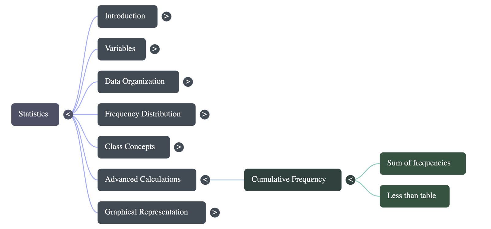
- Definition: Cumulative frequency is a running total. It is the sum of the frequencies of all classes up to and including a specific class.
- Representation: It is often represented in a 'less than' format. For example, "less than 20", "less than 30", showing how many data points fall below that upper boundary.
17.9 Graphical Representation of Data
- Purpose: Reading columns of numbers can be boring and hard to understand. Pictorial or graphical representations are eye-catching, easier to grasp at a glance, and leave a lasting impression on the reader's mind. Graphs must be properly titled and labeled.
17.10 Graphical Representation of Continuous Frequency Distribution
- 1. Histogram:
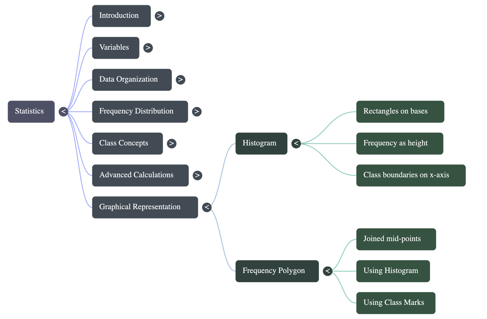
- A graph consisting of touching rectangles. The class-intervals form the bases (x-axis), and their heights match the frequencies (y-axis).
- Important Rule: Data MUST be converted to the exclusive (continuous) form before drawing a histogram.
- The Kink (Zig-Zag line): If the x-axis scale begins at a large number instead of zero (e.g., starting directly at 40), a zig-zag curve or 'kink' is drawn near the origin to indicate the break in the axis.
- 2. Frequency Polygon:
- A line graph obtained by joining the mid-points (class-marks) of the class intervals.
- Method A (With Histogram): Draw a histogram first, mark the top mid-point of every rectangle, and connect them with straight lines.
- Method B (Without Histogram): Calculate the class-marks directly. Plot the class-marks on the x-axis and frequencies on the y-axis, then connect the points.
- Closing the Polygon: To finish the shape, the lines at both ends must touch the x-axis. This is done by joining the ends to the mid-points of imaginary class intervals situated just before the first class and just after the last class (both at a frequency of zero).
Do checkout all questions & answers of this chapter.
Quick Navigation:
| | | |
1 / 1
Quick Navigation:
| | | |